In a previous blog post, we pinned down a definition for mode-covering vs. mode-seeking behavior for distributional divergences. When fitting $q$ to a target $p$, we studied the derivative norm of the divergence wrt $q(x)$ where $p(x) > 0$ and $q(x) \to 0$.

Mode-covering pressure means that when $p(x) > 0$ and $q(x) \to 0$, the gradient of the divergence w.r.t. $q(x)$ diverges strongly (at least $O(p/q)$), pushing $q$ to cover that region.

The forward KL has $O(p/q)$ mode-covering pressure, which is exponentially stronger than the reverse KL with $O(\log(p/q))$ pressure.

In this blog post, we’ll apply our gradient analysis to the Stein discrepancy. We will show that the Stein discrepancy has $O(1)$ pressure (wrt $q$), so mathematically it is even less mode-covering than the reverse KL! Experimentally, we show that Stein discrepancy has a similar loss landscape as reverse KL, and not forward KL.

Stein discrepancy

The Stein discrepancy is a measure of distributional similarity which can be used as a sampler evaluation metric, as it does not require iid samples from the target $p$, or its normalized density. Instead, we can compute it using:

• $\nabla_x \log p(x)$, the data score
• iid samples from $q$

The core object in the Stein discrepancy is the Stein operator, which acts on a vector test function $g(x)$. Using the data score, the Stein operator is:

$$ \mathcal{T}_p g(x) = \nabla_x \log p(x) \cdot g(x) + \text{div}~g(x) $$

This is constructed to satisfy the key property that:

$$ \mathbb{E}_{p}[\mathcal{T}_p g(x)] = 0 $$

for all test functions $g$.

The Stein discrepancy is then defined as:

$$ S(q||p) \triangleq \sup_{g \in G} | \mathbb{E}_{x \sim q} [\mathcal{T}_p g(x)] | $$

where $\mathcal{G}$ must be constrained to keep the supremum finite. One common choice is $\mathcal{G}$ as the unit ball in a reproducing kernel Hilbert space, which corresponds to kernel Stein discrepancy. Another choice is neural Stein discrepancy, where $\mathcal{G}$ is chosen to be the set of functions learnable by a (regularized) neural network.

Mode-coverage pressure analysis via gradient norm

Let’s denote $g_q^*$ as the $g$ that achieves the supremum. Then,

$$ S(q||p) = \mathbb{E}_{q} [ \nabla_x \log p(x) \cdot g^*_q(x) + \text{div}~g^*_q(x) ] $$

Differentiating wrt q, the multiplicative factor of $q$ from the expectation disappears, and we keep the integrand:

$$ \frac{\partial}{\partial q(x)} S(q||p) = \nabla_x \log p(x) \cdot g^*_q(x) + \text{div}~g^*_q(x) $$

Note: This is justified by Danskin’s theorem / the envelope theorem, which says that for some $f(x) = \max_{z} \phi(x,z)$, if the maximizer $z^*$ is unique, then $\frac{\partial}{\partial x} f(x) = \frac{\partial}{\partial x} \phi(x, z^*)$.

Suppose $\mathcal{G}$ imposes bounds $|g|_{\infty} \leq B$ and $| \nabla g |_{\infty} \leq D$, which is a loose assumption satisfied by kernel and neural Stein discrepancies. Then, for any $g$ and all $x$,

$$ \begin{align} | \nabla_x \log p(x) \cdot g(x) + \text{div}~g(x) | &\leq | \nabla \cdot g(x) | + | g(x) | | \nabla_x \log p(x) | \\ &\leq dD + B | \nabla_x \log p(x) |, \end{align} $$

where $d$ is the dimension, and we use the triangle inequality and $| \text{div}~ g| \leq d |\nabla g|_{\infty}$.

In particular,

$$ \frac{\partial}{\partial q(x)} S(q||p) \leq dD + B | \nabla_x \log p(x) |. $$

This is independent of $q(x)$. The pressure term is $O(|\nabla_x \log p(x) |)$.

Thus, the supremum Stein discrepancy, is not mode-covering: it exerts bounded, location-dependent pressure that does not increase when $q(x) \to 0$ in regions where $p(x) > 0$.

Interestingly, the Stein discrepancy at $O(1)$ pressure (wrt q) is even less mode-covering than the reverse KL at $O(\log(p/q))$ pressure!

Experiment

We repeat the common experiment, where our target $p$ is a mixture of two Gaussians with means -4, +4, and std 1. We consider a model distribution $q$ that is a single Gaussian with free parameters mean and std, and plot the divergence/discrepancy between $p, q$ as the mean and std of $q$ vary.

We compute the reverse and forward KL for comparison, and computed Stein discrepancy using kernel Stein discrepancy with an IMQ kernel with $\beta=0.5$, $c=1$, which are common hyperparameter choices.

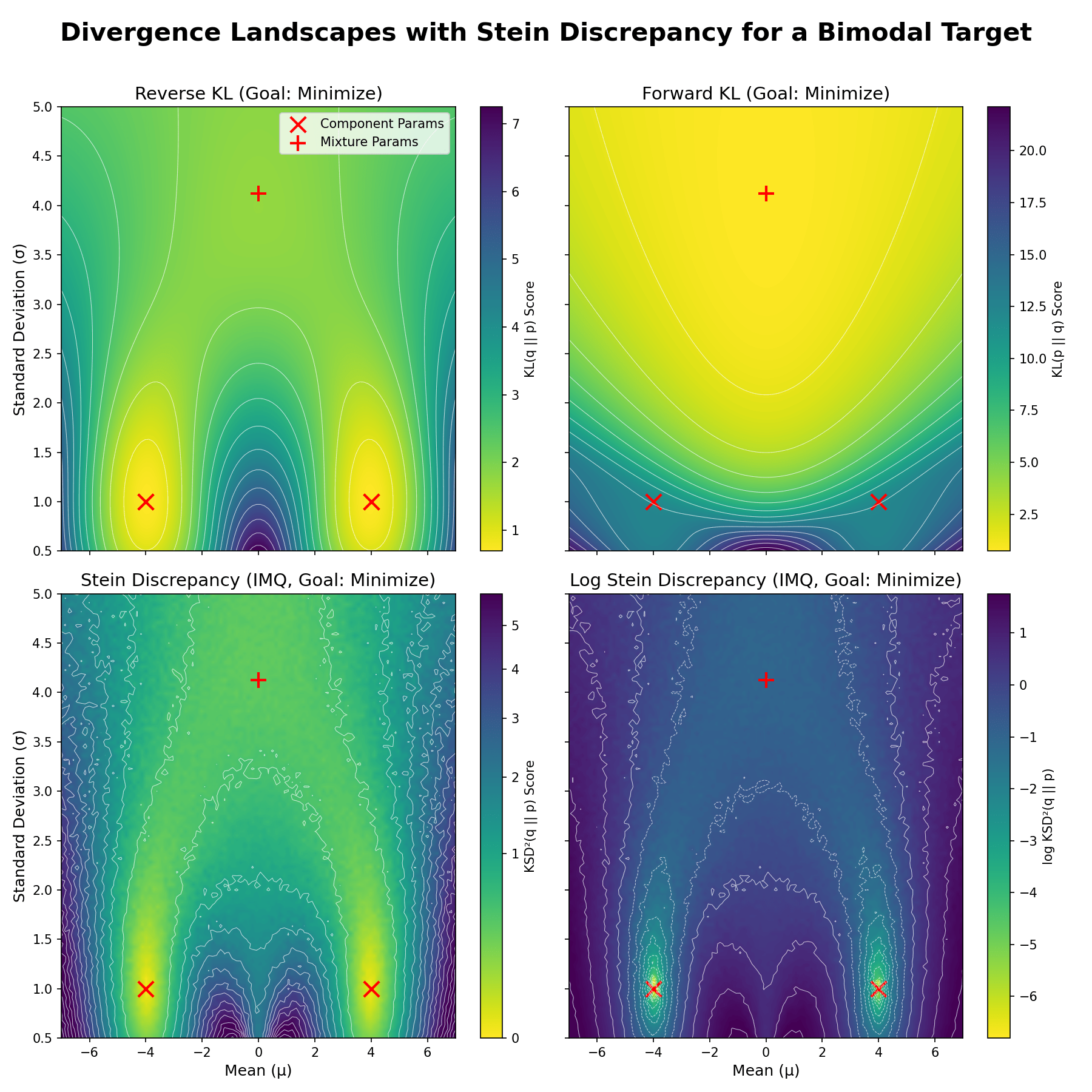
Yellow indicates lower (better) divergence values. The red X’s denote the mean and std of the two Gaussians in the target mixture, while the red + denotes the true mean and std of the target mixture, when fitting a single Gaussian to it.

The top row depicts the reverse and forward KL, and the bottom row depicts the Stein discrepancy and log Stein discrepancy. Visually, the Stein discrepancy’s landscape is similar to the reverse KL: The brightest yellow is at the mode-seeking solutions; the mode-covering solution (red +) is less bright yellow. This relation is more clearly seen on the log scale plot.