What does mode-covering behavior really mean for KL divergence?
We offer a precise definition in terms of the derivative norm of the KL wrt $q(x)$. The forward KL gradient scales as $O(p/q)$, which explodes when $q(x) \to 0$ where $p(x) > 0$, thus strongly encouraging $q$ to cover $p$. In contrast, the reverse KL gradient scales as $O(\log(p/q))$ which is exponentially weaker.
Consider a learned distribution $q$ which we optimize towards a target distribution $p$. The two KL divergences, forward KL and reverse KL, measure how far $q$ is from $p$.
$$ \text{Forward KL}: \quad KL(p||q) = \int p(x) \log\frac{p(x)}{q(x)} dx $$
$$ \text{Reverse KL}: \quad KL(q||p) = \int q(x) \log\frac{q(x)}{p(x)} dx $$
The forward KL is mode-covering, meaning it prefers $q$ which covers all the modes of $p$, even at the cost of being “broader” than p. In contrast, the reverse KL is mode-seeking: it prefers $q$ which is “narrow” and covers a subset of $p$ well.
This has been commonly shown by studying how each KL optimizes a unimodal Gaussian’s mean and std to fit a target distribution that is a mixture of two Gaussians. In this case, the “model” distribution class is not flexible enough to perfectly fit the target.
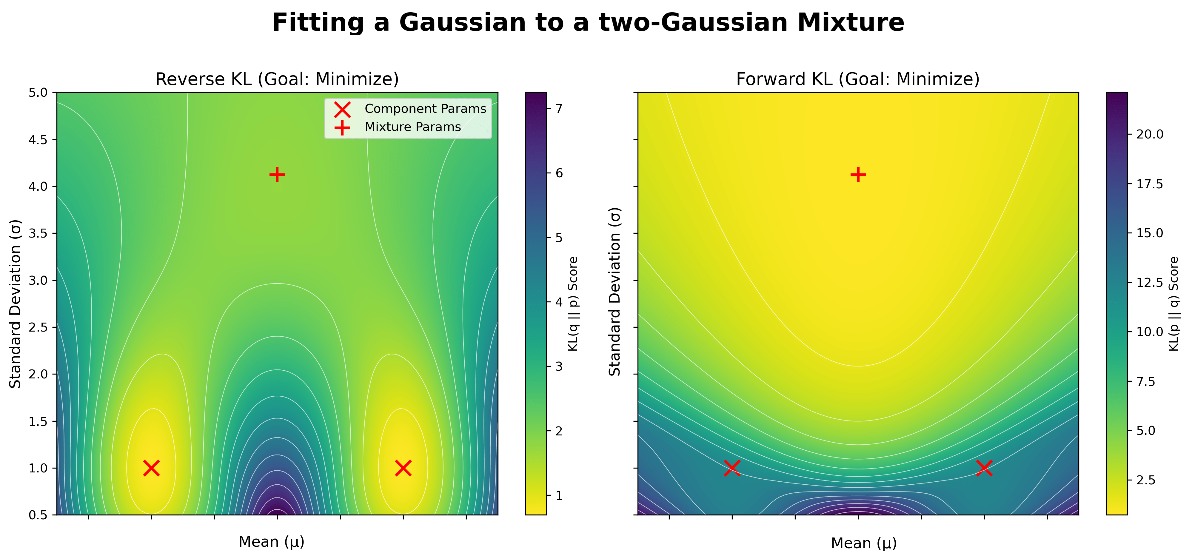
Here, we plot the divergence landscape as a function of $q$’s mean and standard deviation. Yellow indicates lower (better) divergence values. The red X’s denote the mean and std of the two Gaussians in the target mixture, while the red + denotes the true mean and std of the target mixture, when fitting a single Gaussian to it. The optimal model under the reverse KL fits one of the target modes exactly, sacrificing coverage of the other mode, while the optimal model under the forward KL prefers to spread out, placing density over both modes, but sacrificing an accurate fit to either mode.
While this picture provides intuition, it does not provide a precise handle on what mode-covering or mode-seeking behavior really means. A more quantitative approach is to study how much “pressure” is put on the KL score on a point $x$ where $p(x) > 0$ but $q(x) \to 0$. Specifically, let’s look at the partial derivative of the KL wrt $q(x)$:
For the Forward KL, at a given $x$:
$$ -\frac{\partial}{\partial q(x)}p(x) \log\frac{p(x)}{q(x)} = \frac{p(x)}{q(x)} $$
For the reverse KL, at a given $x$:
$$ \begin{align} -\frac{\partial }{\partial q(x)} q(x) \log\frac{q(x)}{p(x)} &= -\frac{\partial}{\partial q(x)} q(x) \log q(x) + \frac{\partial}{\partial q(x)} q(x) \log p(x) \\ &= -\left( 1 \log q(x) + q(x) \frac{1}{q(x)} \right) + \log p(x) \\ &= -\log q(x) + 1 + \log p(x) \\ &= \log \frac{p(x)}{q(x)} + 1 \end{align} $$
The forward KL has derivative norm $O(p/q)$, which explodes as $q \to 0$. This means the forward KL itself increases rapidly as $q \to 0$ wherever $p > 0$. The forward KL is thus penalized heavily for missing any $p$-mass.
In contrast, the reverse KL has derivative norm $O(\log(p/q))$, which is exponentially weaker. The reverse KL is penalized little for missing $p$-mass.
Mode-covering pressure means that when $p(x) > 0$ and $q(x) \to 0$, the gradient of the divergence w.r.t. $q(x)$ diverges strongly (at least $O(p/q)$), pushing $q$ to cover that region.
Armed with this, in the next blog posts we’ll take a look at:
- An impossibility result for sampler evaluation metrics: we cannot have a mode-covering sampler evaluation metric that avoids importance sampling
- We’ll show that the Stein discrepancy is mode-seeking like reverse KL.