[Congress] should be in miniature, an exact portrait of the people at large. It should think, feel, reason, and act like them. – John Adams, Thoughts on Government (1776)

Background

DeepFunding¹ is a proposed system for funding public goods designed around human expert answers to “Did project A or B contribute more to outcome C?”. To scale expensive human expert feedback to many projects and outcomes, DeepFunding uses an open, permissionless collection of AI models which compete in the style of a Kaggle contest or prediction market to best predict human expert comparisons. The AI models are akin to an “engine” which is steered by a small amount of human feedback. The final funding allocation can be a weighted average of model results, weighted by how well models satisfy human expert preferences on held-out validation data.

More broadly, DeepFunding can be viewed as an experiment where humans elect an “AI government body” by voting on AI agents that best satisfy human values. The AI government body is formed as an ensemble of AI agents which represents the humans, while scaling decision-making action to many more issues, topics, and details than the human voter’s may have attention or bandwidth to think deeply about. Yet designing governance structures is tricky: how do we ensure that the ensemble government best represents the potential diversity of human values? While we may look back to the history of human government for insights, the use of AI also introduces novel technical questions and issues: e.g., unlike traditional government, it is possible to have more AI agents than human voters.

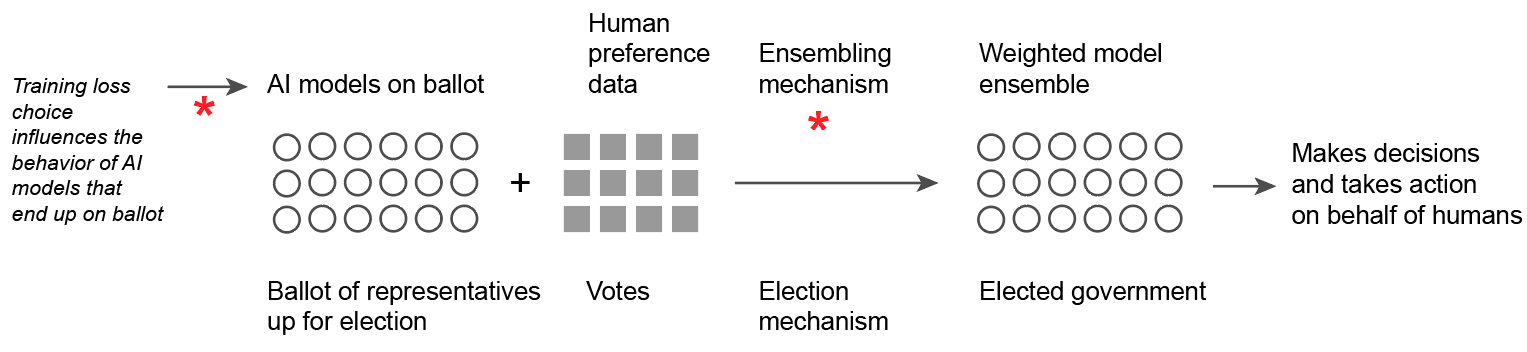
While there are many ways the DeepFunding system can be implemented in detail, the current mechanism² gathers human judgments on project contributions into training and validation datasets. Models are trained on mean-squared error (MSE) loss and submitted in an open, permissionless manner. Each individual model’s quality is measured by training or validation MSE. The ensemble is formed as a weighted mixture models, such that the ensemble minimizes validation MSE, while constraining ensemble model weights to be positive and sum to 1.

The design of the loss function and ensembling method is a key decision point, akin to designing voting and electoral systems, which carries the responsibility of ensuring that human values are captured faithfully by the AI engine or government. In this blog post, I discuss properties of the current ensembling mechanism in DeepFunding, some of which may be undesirable. I highlight a design axis reflecting philosophical values: should we reward centrist models, even if no humans are centrist? This is what MSE rewards. Or should we reward models that accurately capture subsets of human values, and ensemble to express rich distributions of human values?

I suggest the framework of Bayesian model averaging with the sum-Gaussian likelihood (BMA+sumgaussian). In the government analogy, BMA-sumgaussian can achieve proportional representation³ in the elected body. It encourages more model diversity than MSE, and can produce ensembles mixing together models which individually fit well to subsets of expressed human beliefs, and enjoys theoretical optimality properties. As overall ensemble quality increases with model diversity, this also serves to improve alignment between individual model developer goals (training loss) with overall ensemble quality.

Importantly, BMA+sumgaussian is simple: I implement it in negative lines of code compared to the current DeepFunding ensembling code, and it changes only 1 line of code in loss functions for training and validation. Furthermore, it can be applied retrospectively or in parallel to the existing DeepFunding mechanism, so it can be evaluated without protocol changes.

Summary for ML folk: I propose Bayesian model averaging with the sum-Gaussian likelihood as an ensembling solution for this problem setting, which is characterized by several interesting properties:

• The many-model ensembling problem setting, with more models than validation datapoints. This setting is unusual in conventional ensembling, where we typically have few models and lots of validation data.
• We assume that label distributions can be meaningfully bimodal or multimodal, as they reflect human values. This richness is captured by the sum-Gaussian likelihood, which is equivalent to an RBF kernel density estimate on labels.
• Overall ensemble quality benefits from diverse models. We desire a measure of individual model quality (a training objective) which encourages model diversity, without having to see other models. This challenge arises because unlike conventional ensembling where we control all model training, here, models come from a Kaggle contest. For the sanity of individual model developers and the leaderboard, we’d like model quality metrics to be a fixed function of the dataset. This excludes methods like correlation penalties⁴ which depend on the full model collection, which varies over time.

Overview

We observe several properties of the current ensembling mechanism:

• Increasing number of models can be problematic. When the number of models exceeds the number of human expert validation datapoints (the “many-model ensembling” problem), the ensemble weights can be underdetermined, which means many funding allocations are equally consistent with human preference data. The final funding allocation on unseen projects depends on a tie-breaker, which can potentially be arbitrary. If the current implementation persists, I recommend being explicit, rather than implicit, about the tie-breaker mechanism. This is a realistic situation in DeepFunding, which aims to use a small amount of human expert labels, and encourages many models to be submitted in an open, permissionless manner: mini contest #2 reached over 1,000 model submissions in less than 24 hours from launch⁵.
• Perhaps counterintuitively, higher individual model quality assessed by validation MSE does not guarantee higher weight in the ensemble (though it is correlated). I prove this by simulation. This means models that better fit the human preference data, can be weighted less in the ensemble for final funding allocation, than worse-fitting models. The worse-fitting models can thus have a larger impact on final funding allocation on unseen projects.
• Under MSE loss, individual models are rewarded for being centrist, which is misaligned with overall ensemble quality which benefits from diversity in models. Furthermore, MSE incentivizing centrism is problematic if human value judgments are bimodal: centrist models are rewarded even if no humans have centrist values, whereas models are penalized for more accurately capturing either human extreme.

I suggest an alternate scoring mechanism using Bayesian model averaging (BMA), which takes model weights as $p($model | human validation data$)$ to form an ensemble. BMA resolves aforementioned issues. In BMA, the individual model quality metric is directly its ensemble weight, so higher quality models that better fit the human preference validation data are always assigned greater weight. Ensemble weights are always determined, even if there are more models than validation datapoints. The BMA ensemble is optimal in minimizing KL-divergence to the “true” label distribution, among all ensembles in the hypothesis set. Finally, BMA with the sum-Gaussian likelihood incentivizes model diversity by rewarding models for matching subsets of human preferences well, rather than being centrist. As ensemble quality benefits from model diversity, this helps aligns individual model developer goals towards improving overall ensemble quality.

Details

The remainder of this article is structured as a “bullet point list” of focused sections, where each section dives into a particular statement. Sections are separate, can be read in any order, and elaborate on particular points in the higher-level summary.

The underdetermined case (the “many-model ensembling” problem)

The validation data of human expert judgments are represented as a vector $\mathbf{y} \in \mathbb{R}^{N}$ on $N$ project comparisons, where each entry holds the human-labeled log value of some project B over A for outcome C. For $D$ models, the matrix $\mathbf{X} \in \mathbb{R}^{D \times N}$ holds the predictions of each model for each project comparison in the validation set. The current scoring mechanism finds weights $\mathbf{w} \in \mathbb{R}^D$ by constrained least-squares regression:

$$ \min_\mathbf{w} | \mathbf{w}^\intercal{}\mathbf{X} - \mathbf{y} |_2^2 \qquad{} \textrm{s.t. } \mathbf{0} \leq \mathbf{w} \leq \mathbf{1} , \sum_i w_i = 1. $$

When $N < D$, that is the number of human-labeled validation project comparisons is fewer than the number of models, $\mathbf{w}$ can be underdetermined, meaning there is an infinite number of distinct models weights that all satisfy the human preference labels optimally. This can be problematic because distinct optimal ensembles can have different funding allocations on unseen projects, but the human labels are insufficient to pin down one exact ensemble. Thus, a tie-breaker is required to finalize funding allocation.

In the current code (reproduced below), scipy.minimize is used to solve the constrained optimization problem. I’ve found empirically through some light testing that when solving an underdetermined constrained problem, scipy.minimize returns the vector closest to the initial guess. So the current code’s tie-breaker chooses the model weights closest to uniform. If the current implementation persists, I recommend making this behavior explicitly documented as intentional, rather than implicit as its current state is. Very light $L_2$-regularization (i.e., with weight 1e-6), is also a good approach to break ties more explicitly without harming ensemble fit.

 1
 2
 3
 4
 5
 6
 7
 8
 9
10
11
12
13
14
15
16
17
18
19
20
21
22
23
24
25
26

def find_optimal_weights(logits_lists, samples):

    def split_cost(weights):
        combined_logits = [
            sum(w * L[i] for w, L in zip(weights, logits_lists))
            for i in range(len(logits_lists[0]))
        ]
        return cost_function(combined_logits, samples)

    # Initial guess: equal weights
    initial_weights = [1 / len(logits_lists)] * len(logits_lists)

    # Constraint: weights must sum to 1
    constraints = ({'type': 'eq', 'fun': lambda w: sum(w) - 1})

    # Bounds: weights must be between 0 and 1
    bounds = [(0, 1)] * len(logits_lists)

    # Minimize the split cost
    result = minimize(
        split_cost,
        initial_weights,
        bounds=bounds,
        constraints=constraints
    )
    return result.x

For DeepFunding, the underdetermined situation is a realistic scenario. Human expert labels are considered expensive, and a goal is to minimize this work (minimize $N$). However, many models can be submitted in DeepFunding’s open, permissionless model marketplace, and DeepFunding appears to encourage this (increasing $D$). For instance, mini contest #2 reached over 1,000 model submissions in less than 24 hours from launch.

It is interesting to speculate that in an AI-agent abundant world, the many-model ensembling problem setting may become more common, when diverse, high-quality models are easy to obtain in abundance, and we aim to steer them with limited human feedback in increasingly varied tasks.

Better individual models (by validation MSE) does not guarantee higher ensemble weight

In this colab notebook⁶, I randomly simulate $n=10$ validation datapoints and $d=5$ models, and fit the MSE ensemble by constrained least-squares regression. I then compare each individual model’s MSE loss to its weight in the ensemble. Recall that in the context of DeepFunding, individual model MSE measures each model’s quality of fit to validation data of human judgments. Through simulation, I find that:

• About 20% of the time, a worse model is assigned higher model weight than a better model
• About ~1% of the time, the learned model weights successfully sort all five models by individual model MSE.
• The average Spearman correlation between individual model MSE and ensemble weight is -0.70. A perfect correlation is -1.0 (lower model MSE always gets higher ensemble weight).

In some failure cases, poorer-fitting models are assigned over 2x higher weight in the ensemble than better-fitting models.

A limitation of this analysis is the use of random vectors, but the fact remains that nothing enforces the optimal least-squares ensemble weight to respect individual model MSE.

Least-squares ensembling finds model weights that all work together well. Each model’s weight can be somewhat interpreted as its contribution in improving the overall ensemble given all other models, when all other model’s ensemble weights are frozen at their optimum. Thus, models that “fix” mistakes in all other models can be rewarded highly. This is a nice property and can help to incentivize models that cover gaps in the model collection, but if it’s not communicated clearly, it might lead to unpleasant surprises.

Ideally, we might like to directly train individual models to maximize contribution to the ensemble, but in the MSE approach, this objective is unstable and unsuitable for individual model development or leaderboard tracking, as it can change over time as the model collection changes.

Bayesian model averaging

In Bayesian model averaging, a collection of models are weighted by their posterior probability given data: $p($ model | validation data $)$, which is calculated by Bayes rule:

$$ p( \textrm{model} | \textrm{validation data}) = \frac{ p(\textrm{validation data} | \textrm{model}) p( \textrm{model}) }{ \sum_i p(\textrm{validation data} | \textrm{model}_i) p( \textrm{model}) } $$

By using a uniform model prior so that all models are equally likely under $p($model$)$, we simplify to:

$$ p( \textrm{model} | \textrm{validation data}) = \frac{ p(\textrm{validation data} | \textrm{model}) }{ \sum_i p(\textrm{validation data} | \textrm{model}_i)} $$

which we can calculate with access to the likelihood function $p($ validation data | model $)$. By dividing by the sum of likelihoods across models, weights are positive and sum to 1.

Currently in DeepFunding, models only produce point predictions: i.e., model(x) $\rightarrow$ y $\in \mathbb{R}$. For compatibility with point-prediction models, I recommend defining a single likelihood function to be shared by all models.

The likelihood function defines what “good model fit” means by determining the “reward” that models receive. Thus, the choice of likelihood function is a key design decision point. In the government analogy, the likelihood function is the election mechanism, responsible for converting votes into an elected body. In the next section, I discuss and recommend the sum-Gaussian likelihood.

Once a likelihood function is chosen, we use it to compute $p($ validation data | model $)$. To obtain predictions from the ensemble with point-prediction models, we use the weighted mixture of model predictions:

$$ \sum_i p( \textrm{model}_i | \textrm{validation data}) \textrm{model}_i(x) $$

Notes

• Bayesian model averaging is optimal in the sense it finds the ensemble whose predictive distribution⁷ minimizes KL-divergence to the “true” label distribution, among all ensembles in the BMA hypothesis set. Notably, this is a different optimality measure than least-squares regression, which minimizes $L_2$ distance between the weighted point predictions to observed points.
• Ensemble weights are directly proportional to $p($ validation data | model $)$, which is the primary quality metric measuring how well the model fits the validation data.
  • Better-fitting models always receive higher weight in the ensemble.
  • This measure of model quality only depends on the validation data and the model, so it is an appropriate metric for model developers and leaderboard ranking
• Each model’s weight in the ensemble is determined only by the individual model and the data, only relying on other models for normalization to sum to 1. Ensemble weights are thus well-behaved and unique even when models outnumber data.

Sum-Gaussian likelihood supports multimodal posteriors, while MSE promotes centrism

Denote the human log-value ratings for a particular project comparison $x$ as $y_1, y_2, …, y_m$. We propose the sum-Gaussian likelihood, parametrized by mean $\mu$, standard deviation $\sigma$, to define the probability of validation data given a model prediction $f(x)$ as:

$$ p(y_1, y_2, …, y_m | \mu = f(x), \sigma) = \frac{1}{m}\sum_i^m \mathcal{N}(y_i | \mu = f(x), \sigma) $$

which contrasts with the standard Gaussian likelihood on multiple samples:

$$ p(y_1, y_2, … y_N | \mu, \sigma) = \prod_i^N \mathcal{N}(y_i | \mu, \sigma) $$

The sum-Gaussian replaces the product with the sum. For a fixed dataset $\mathbf{y}$, the likelihood function $\ell(\mu = f(x) | \mathbf{y})$ is equivalent to an RBF kernel density estimate of the human label distribution. Another view is that it places a Gaussian distribution at each human label, and sums over them.

Importantly, the sum-Gaussian rewards high likelihood to model predictions that match any of the modes of the human label distribution.

Example

Consider a hypothetical example where 5 humans rated +1 (project B > A) and 5 humans rated -1 (B < A).

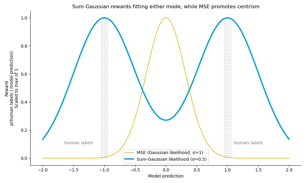
Using MSE, which corresponds to standard Gaussian likelihood, rewards the middle-ground, centrist prediction of zero (project A contributed the same as B) even though no humans were centrist. Under mean-squared error, predicting the average label is optimal. Predicting -1 or +1 receives little reward, even though in a sense this more accurately reflects the two extreme subpopulations.

With the sum-Gaussian likelihood, models are rewarded for predicting either -1 or 1, and receive less reward for being centrist. The sum-Gaussiam likelihood thus is a tool to express the value, or concept, that accurately predicting an opinionated subset of human values is what makes a model desirable.

When the human label distribution is unimodal, the sum-Gaussian likelihood effectively reduces to the standard Gaussian likelihood.

When the human label distribution is bimodal or multimodal, MSE incentivizes conformity and uniformity, as all models aspire to the single optimal solution of predicting the average label. In contrast, with the sum-Gaussian likelihood, there can be multiple high-reward solutions that models can aspire to, which can serve to increase model diversity. This more effectively captures the richness and diversity in complex human label distributions, provides humans with a greater variety of candidate representatives, and strengthens overall ensemble quality.

Further, when human label distributions are bimodal or multimodal, but also unbalanced, the sum-Gaussian likelihood rewards satisfy proportional representation: model likelihood at a mode is directly proportional to the fraction of human labels at that mode. This can help achieve elections (ensembles) satisfying proportional representation.

Training and validation loss under sum-Gaussian likelihood

Mean-squared error is a simple loss function for training models under Gaussian likelihood, because squared distance is proportional to Gaussian log-likelihood: $\log p(y_1, y_2, …, y_m | f(x)) \propto \sum_{i}^m (y_i - f(x))^2$.

Sum-Gaussian likelihood also admits a simple loss function which can be used in place of MSE:

1
2
3

def sumgaussian_loss(pred: torch.tensor, labels: torch.tensor, sigma: float = 0.5):
    squared_error = ((pred - labels) / sigma)**2
    return -1 * torch.logsumexp(-0.5 * squared_error, dim=0)

This corresponds to the sum-Gaussian log likelihood:

$$ p(y_1, y_2, …, y_m | \mu = f(x), \sigma) = \frac{1}{m}\sum_i^m \mathcal{N}(y_i | \mu = f(x), \sigma) $$

$$ \log p(y_1, y_2, …, y_m | \mu = f(x), \sigma) = \log \left( \frac{1}{m}\sum_i^m \frac{1}{\sigma \sqrt{2\pi}} \exp \left( -\frac{1}{2} \frac{(y_i - f(x))^2}{\sigma^2} \right) \right) $$

$$ = c + \log \left( \sum_i^m \exp \left( -\frac{1}{2} \frac{(y_i - f(x))^2}{\sigma^2} \right) \right) $$

where $c$ is a constant that doesn’t depend on the data or the model, and thus is safely discarded in the python code.

Python code: Ensembling with BMA + sumgaussian

 1
 2
 3
 4
 5
 6
 7
 8
 9
10
11
12
13
14
15
16
17
18
19
20
21
22
23
24
25
26
27
28
29
30
31
32
33
34
35
36
37
38
39
40
41
42
43
44
45
46
47
48
49
50
51
52
53
54
55
56
57
58
59
60
61
62
63
64
65
66
67
68
69
70
71
72
73
74
75
76

import numpy as np
from dataclasses import dataclass
from scipy.stats import norm
from scipy.special import logsumexp


@dataclass
class HumanPairData:
    item_index_a: int
    item_index_b: int
    log_value_b_over_a: list[float]


def log_prob(
    model_logits: list[float], 
    human_pair_data: HumanPairData, 
    scale: float = 0.5,
) -> float:
    """ Returns log p(human_pair_data | model_logits) under
        the sum-gaussian likelihood. 

        Parameters
        -----
        model_logits: (num_items)
            Each element i is the logit predicted by the model for item i.
        human_pair_data: HumanPairData
            A list of human preference labels (in log values) of item b over a.
        (Optional) scale: float
            Standard deviation
    """
    a, b, human_log_values = human_pair_data
    model_log_ratio = model_logits[b] - model_logits[a]
    return np.log(np.mean(
        [norm.pdf(human_label, mean=model_log_ratio, scale=scale)
         for human_label in human_log_values]
    ))


def find_bayesian_model_weights(
    all_model_logits: list[list[float]], 
    all_human_pair_data: list[HumanPairData]
) -> list[float]:
    """ Computes posterior probabilities for Bayesian model averaging.

        Calculates p(model | data) ∝ p(data | model) assuming a uniform prior
        over models. The likelihood p(data | model) is computed as the product
        of probabilities for each human preference pair (see log_prob function).

        Parameters
        -----
        all_model_logits : list[list[float]]
            Matrix of model predictions. Shape: (num_models, num_items)
            Each row contains one model's predicted log-values for all items
        all_human_pair_data : list[HumanPairData]
            List of human preference data for different item pairs.
            Each element contains indices of compared items and human labels

        Returns
        -------
        list[float]
            Posterior probabilities for each model. Shape: (num_models)
            Values are in [0,1] and sum to 1

        Notes
        -----
        - Assumes uniform prior over models
        - Uses log-space computations for numerical stability
        - Models with predictions closer to human preferences receive higher weights
    """
    def model_logprob(model_logits: list[float]):
        return sum(log_prob(model_logits, human_pair_data)
                   for human_pair_data in all_human_pair_data)

    model_logprobs = [model_logprob(model_logits) for model_logits in all_model_logits]
    model_weights = np.exp(model_logprobs - logsumexp(model_logprobs))
    return model_weights

References

https://github.com/deepfunding. Discussions on existing mechanism are based on the repository accessed on 1/14/25. ↩︎
https://www.nytimes.com/interactive/2025/01/14/opinion/fix-congress-proportional-representation.html ↩︎
https://blog.blackhc.net/2022/10/diversify_active_learning_and_ensembles_via_BALD/ ↩︎
https://colab.research.google.com/drive/1agbgeU0zDLkIAGLzkg_ZiQxirDFd4a8S ↩︎
When models only output point predictions (i.e., models are not inherently probabilistic), the BMA predictive distribution depends on how the likelihood is defined. In general, the posterior predictive distribution is $p(y’ | \mathbf{y}) = \sum_i p(y’ | \textrm{model}_i) p(\textrm{model}_i) | \mathbf{y})$, where $y’$ is unseen data, and $\mathbf{y}$ is the seen dataset. Under the sum-Gaussian likelihood, when $y’$ is a single sample, the posterior predictive distribution is a mixture of Gaussians. ↩︎